Tips and tricks in R

Maria Bobrowski | Niels Schwab | Charlotta Mirbach
RLab - Skriptbasierte modulare Umweltstatistik (Universitätskolleg 2.0)
Universität Hamburg
RLab-Impressum
Gefördert im Rahmen des „Lehrlabors“ im Universitätskolleg 2.0 aus Mitteln des BMBF (01PL17033)

Dieses Digitale Skript von Niels Schwab, Maria Bobhrowski und Charlotta Mirbach, Universitätskolleg 2.0 / Lehrlabor, Universität Hamburg, ist lizenziert unter einer Creative Commons Namensnennung - Weitergabe unter gleichen Bedingungen 4.0 International Lizenz.
elearn.js Template
Universität Hamburg
Das elearn.js Template von Universität Hamburg ist lizenziert unter einer Creative Commons Namensnennung - Weitergabe unter gleichen Bedingungen 4.0 International Lizenz
Objective
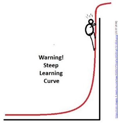
In order to overcome the extremely steep learning curve, some hints, tips and tricks have been compiled on the following pages to make learning R easier for you:
- Comparision of GUI and IDE
- Updating of R, R-packages and RStudio
- Saving results from the environment and from the console
- Saving plots
- Tips and tricks to save tables
- The art of scripting
- Example R-script
- Adding comments to your code
- R cheat sheets
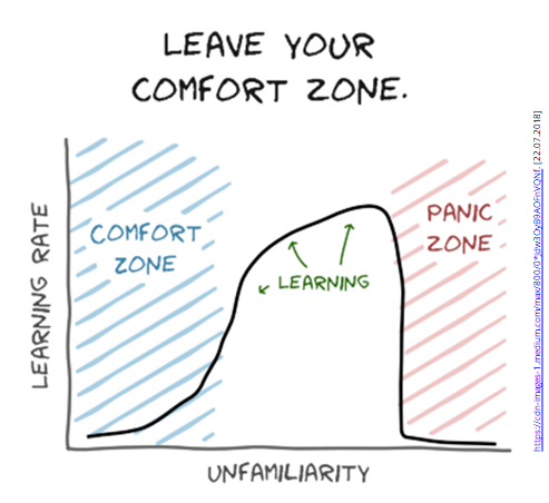
As you learn new skills, you will sooner or later face challenges. The same goes for learning a new language - in your case the programming language R.
Look at it as an exploratory tryout of a new environment.
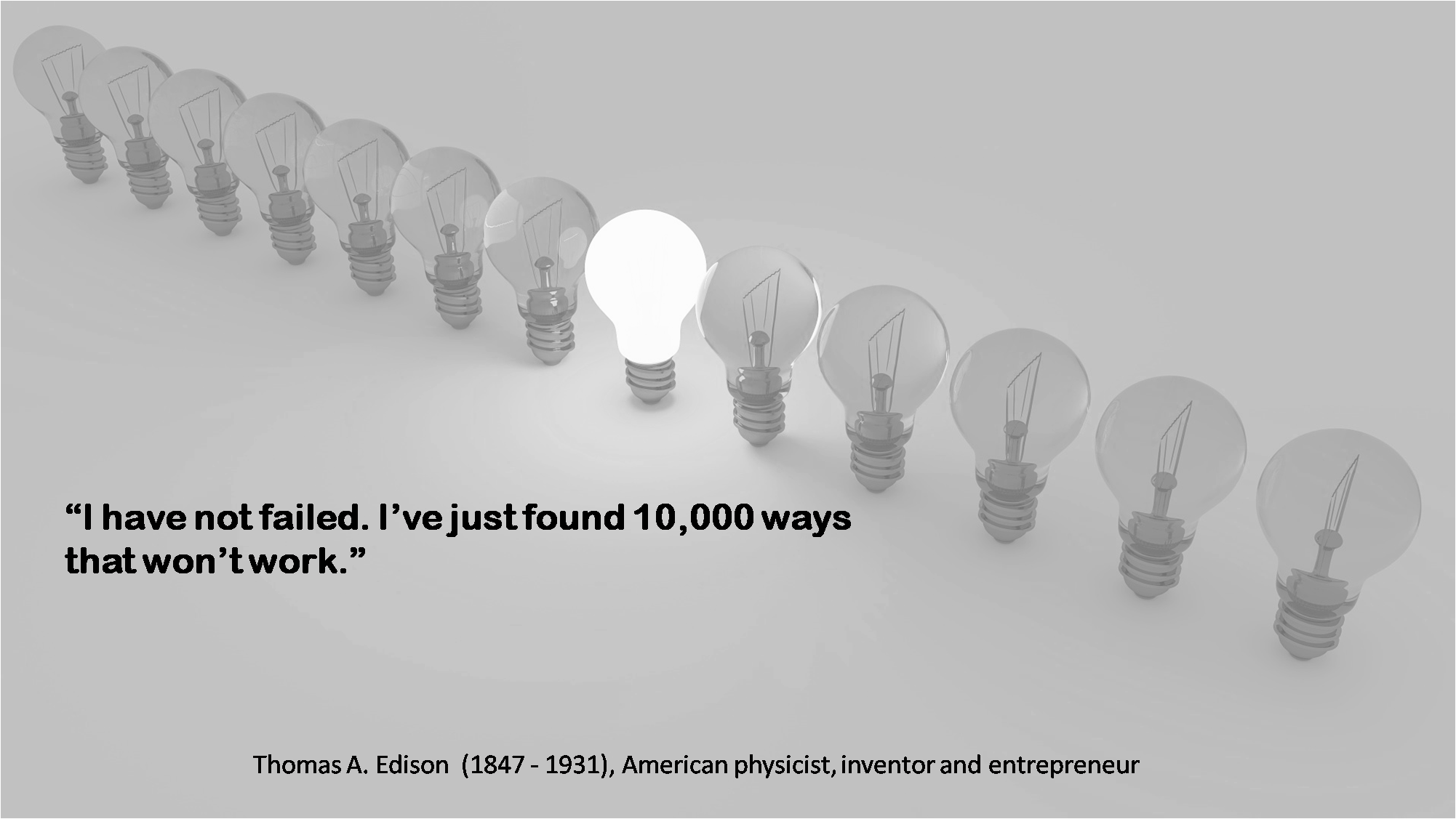
Don't be confused by error messages! Better think as Thomas A. Edison, the inventor of the light bulb, said:
Prerequisites
To understand this script, you should have
- R and RStudio installed and
- connected R to RStudio and
- you should be familiar with the four windows of RStudio.
All this is described in the digital scripts How to install R and RStudio and RStudio und R-Skripte (the latter in german only), look there if necessary and then return here!
It is best to open RStudio parallel to the digital script, so that you can try out the functions directly. You can also read the digital script on a smartphone or tablet.
Questions or remarks?
The RLab team is always grateful for suggestions and comments to improve this digital script! You can also ask questions about the content! Use the comments for all this!
GUI versus IDE
Especially when you are learning R at the beginning, the script-based control and the endless possibilities of statistical analysis can be intimidating. Compared to other statistical software such as Excel or SPSS, RStudio does not have a Graphical User Interface (GUI), but an Integrated Development Environment (IDE).
MS Excel, SPSS, ...? BetteR use R! :)
Compared to the pure program R, RStudio provides you with the script window, plot window, environment and console to make it easier to use. However, it is a prerequisite that you know in advance what you want to calculate or display. In RStudio there is no possibility to "click" through the choices as in e.g., SPSS.
The control of the program R is script-based and it is important that you don't get discouraged by error messages. It is quite normal for error messages to appear or for something not to work as intended.
For general information on R-Help functions, see the digital script R-Hilfe in- und außerhalb von R (in german only).
Installing an R package
Here you can see how easy and quick you can add an R package to your R installation!
-
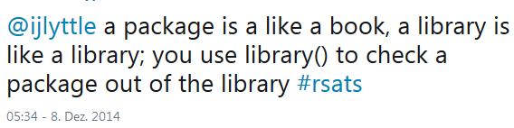
R packages make R special: There are thousands of freely available packages and the enormously high functional range of R is achieved with them. A package is a kind of add-on module that is integrated into R (figure source: Quote of Hadley Wickham at twitter.com).
-
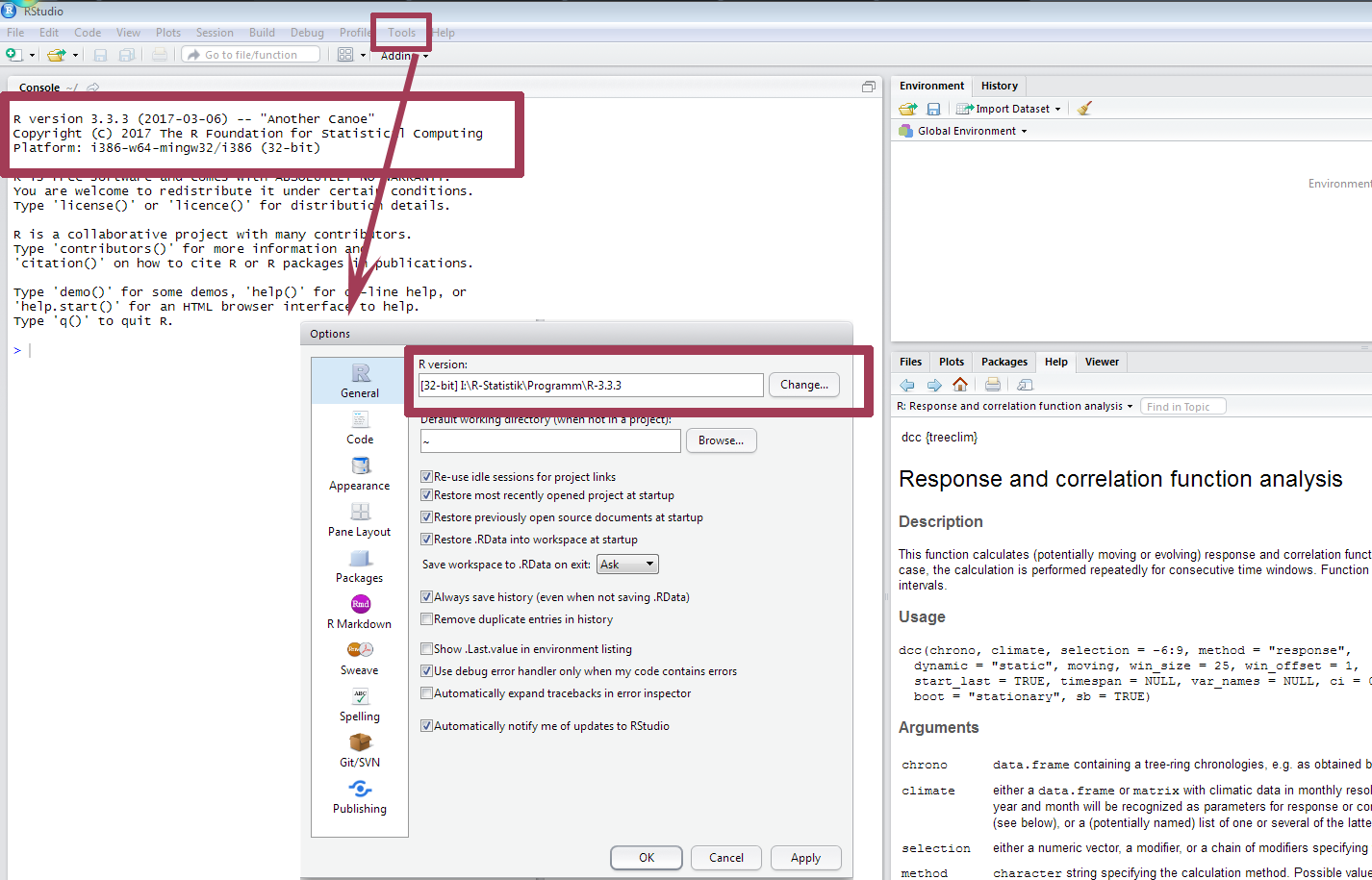
Before installing an R-Package a short check: It may be possible that different R-versions are installed on your computer. To install the R-Package into the "Package Folder" (Library) of the version you are using, you should check if RStudio is connected to the correct R-Version. How to do this is described in detail in the Digital Script How to install R and RStudio.
-
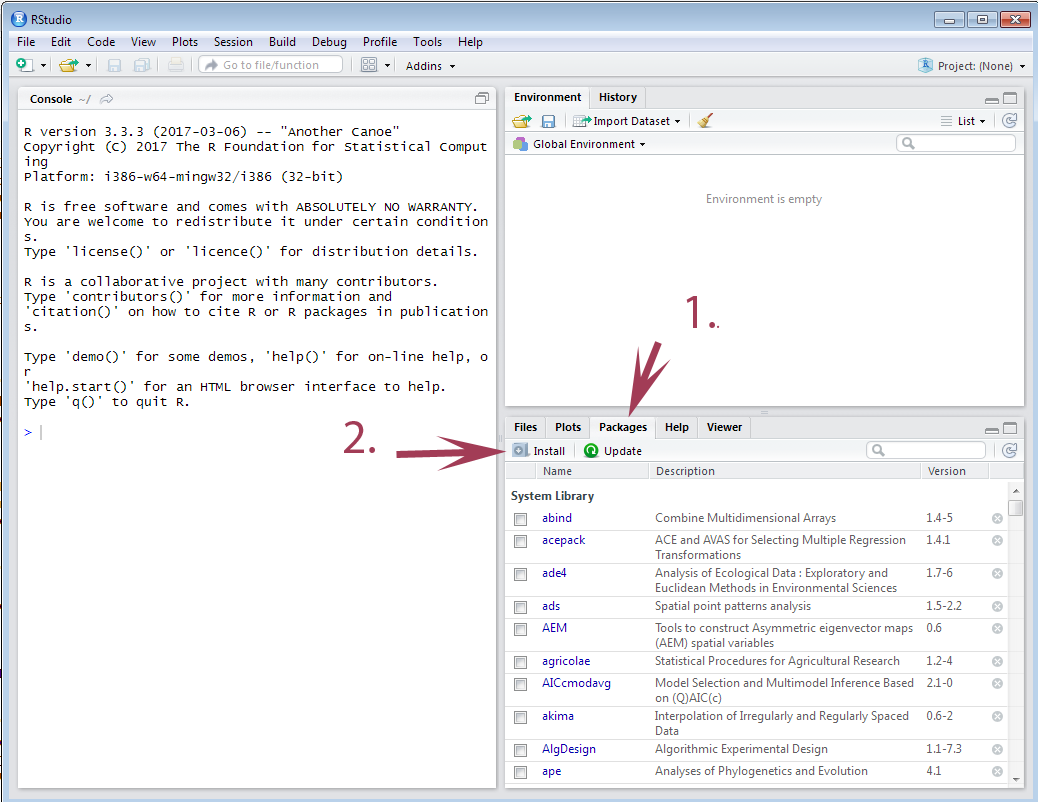
To install a new R Package, simply click on the "Install" button in the RStudio tab "Packages".
-
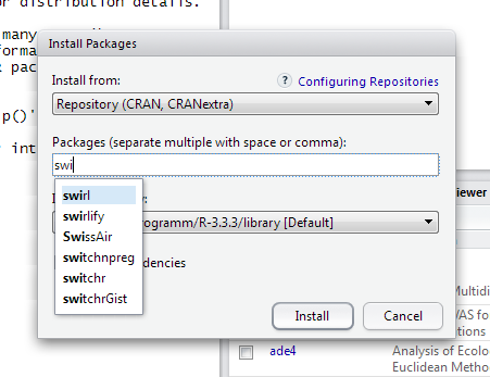
In the window that opens, enter the name of the package (here: swirl). You can then choose from which server the package will be loaded. Now at the latest you need an internet connection. Usually all settings in this window are ok, you can simply click "Install".
-
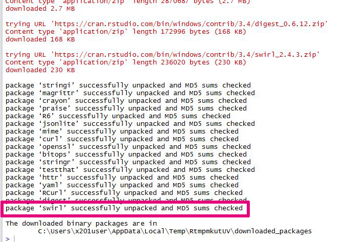
After clicking "Install" some things should happen: Some lines of code appear on the left, in the so-called console. If the desired package depends on others, these packages will be installed automatically. The successful installation of the package (swirl in this case) can be recognized by the message "package 'swirl' successfully unpacked and MD5 sums checked" appearing in the console, no error message is present and....
-
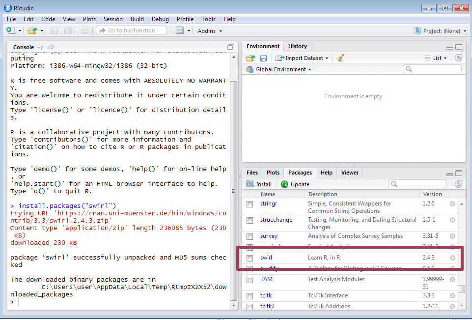
... "swirl" is displayed in the list of installed packages. If this doesn't work so far, you can ask a question as a comment or ask the course administration in a classroom course!
Another option to install packages is to includeinstall.packages("package name 1", "package name 2", "....")in your R code. This may have advantages and disadvantages, depending on your way to work, purpose of your code etc. At least theinstall.packages()code should be commented out to avoid reinstalling the package every time you run the code.
Background information about R-Packages:
- Álvarez, A. / DataCamp (2017) R Packages: A Beginner's Guide [accessed March 26, 2019]
- CRAN Contributed Packages [accessed March 26, 2019]
- Grolemund, G. / RStudio Quick list of useful R packages [accessed March 26, 2019]
- Wickham, H. (2018) R packages book [accessed March 26, 2019]
Questions or remarks?
The RLab team is always grateful for suggestions and comments to improve this digital script! You can also ask questions about the content! Use the comments for all this!
Updating R, R-packages and RStudio
The R Core Team is responsible for R and is posting new R versions regularly. To be always up to date, you can use the function updateR(). It is included in the "installr" R package. updateR() automatically searches for the latest R version and then offers the possibility to install it. So you are always up to date!
Although administrator rights are required for the first installation of R and RStudio, they are not required when updating the programs.
install.packages("installr")      # installing the package
library(installr)                 # activating the package

updateR()                         # searching for recent version
If you are up to date with your R version, FALSE will be displayed in the console.
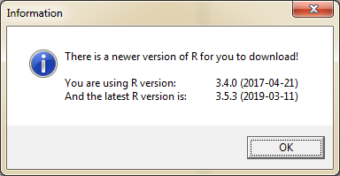
If you are not up to date with your R version, a new window will appear. In this case the latest R version is 3.5.3.
In the next step a new window will appear asking you if you want to see the news about this version.
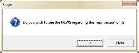
If you click on "Yes", the website opens with the news about the latest R version. Here are the information, respectively the updates of the version summarized. These news are same as at the download page's "New features in this version"-section.
To install the latest version of R, click "Yes" in the following dialog.
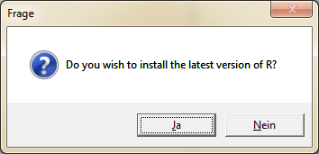
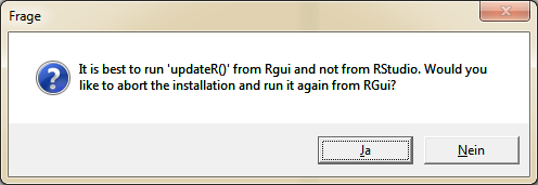
To install the latest R version without leaving RStudio, click "No" in the next step.
This is followed by the R installation process. No administrator rights are required.
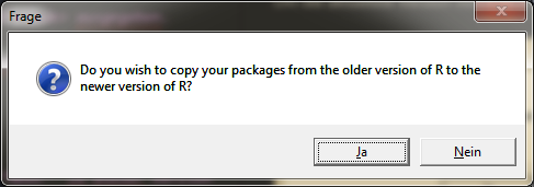
After the installation process is complete, a new window will appear asking if you want to copy the packages from the old R version to the new R version.
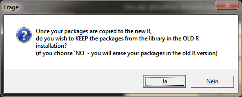
Here you can decide if you want to keep the packages in the old R version or not.
Warning! The copy process may take a while, depending on how many packages are contained in the R Library.
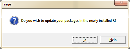
When the copy or move operation is finished, the question for the update of the packages appears.
Once this process is complete, you must select the "new" R version in the global options. Then close RStudio once and open it again.
Well done! You are up to date with your R version and your R packages!
To avoid error messages, it is recommended to delete the *"old"* version from your pendrive or hard disk.
Want to update RStudio?
The function install.RStudio() updates your RStudio version. You can also find this function in the package "installr".
Note: The function does not check the currentness of your version, but simply overwrites the existing version.
Saving results
How can the results of an analysis or a calculation be saved in order to work with them at a later time?
How can results be written out of R so that they can be further processed in another program?
The data must be storedIn the following we will deal with the storage and loading options of:
- all objects in the environment
- output in the R console
Saving objects from the environment
You may have noticed when closing R that you are asked if you want to back up the workspace. This file has the extension .RData.
The following screenshot will look familiar to you.
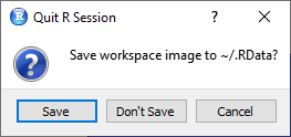
If you click on save here, your entire workspace will be saved where your working directory was set. In this case, the working directory was not set, so the workspace was saved on the computer in the documents directory.
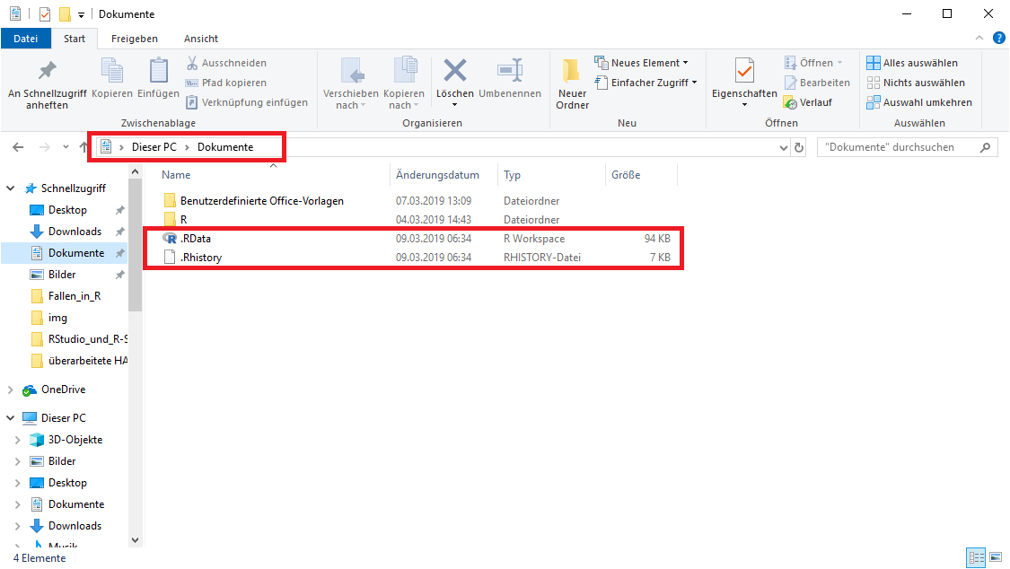
This procedure has several disadvantages:
- If you save without the "correct" file name, it will be difficult for you to reassign the saved content of this file to the corresponding script.
- If you reopen R and RStudio, the file in that location will automatically reload into the environment. The reason for this is that all files are loaded from this directory. The packages are also stored here.
- When a workspace is saved again, the previous file is overwritten without a warning message.
- If you are working at university computers, you might not be able to find your file again once the computer has been shut down. These computers might be configured so that all files that have not been saved in the course directory are deleted on shutdown.
Best practice
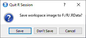
The function save.image() is used to store the entire environment i.e., the workspace (internal memory of R). Here you can specify the storage path and also a file name
save.image("F:/R/results_correlation/correlation.RData").
It is recommended to copy this code snippet to the end of each script. So you always have the possibility to save your workspace.
Setting a working directory can save results. So the workspace will at least be saved in the corresponding directory when you close it.
Loading Objects into the Environment
To reload the workspace into R the function load() is used.
load("F:/R/results_correlation/correlation.RData")You open RStudio and there are already files in the environment?
A workspace (.RData) has been loaded.
With the function rm() you can delete (rm = remove) all files at once in the environment.
rm(list = ls()) # deletes everything in environment/workspacesThis action cannot be undone.
Again, it is recommended to copy thisSaving console output
To save the structure of an object, you can write the whole console output to a file with the function sink(). This can then be opened for example with the editor and further processed. The function sink() redirects the output of the console to a file. During the active redirection, the output is only to the output file and no longer to the console. With the repeated function sink() the redirection is deactivated and the output takes place again in the console.
sink("F:/R/results_correlation/correlation..txt") # redirection activated
                                # setting file name and file extension
cor(sat.act[1:200,2:3] )        # without previous setting, result would be written to console
sink()                          # redirection deactivated
file.show("Korrelation.txt")    # showing file in new window
Saving plots
Just like tables and other results, graphics have to be savedThe following section introduces you to 2 ways to export graphics you have created from RStudio.
Saving via the IDE (Integrated Development Environment)
In RStudio there is the possibility to export created plots via the plot window via the menu item "Export". Here you can choose between different file formats.
You can see a step-by-step guide in the following slideshow:
-
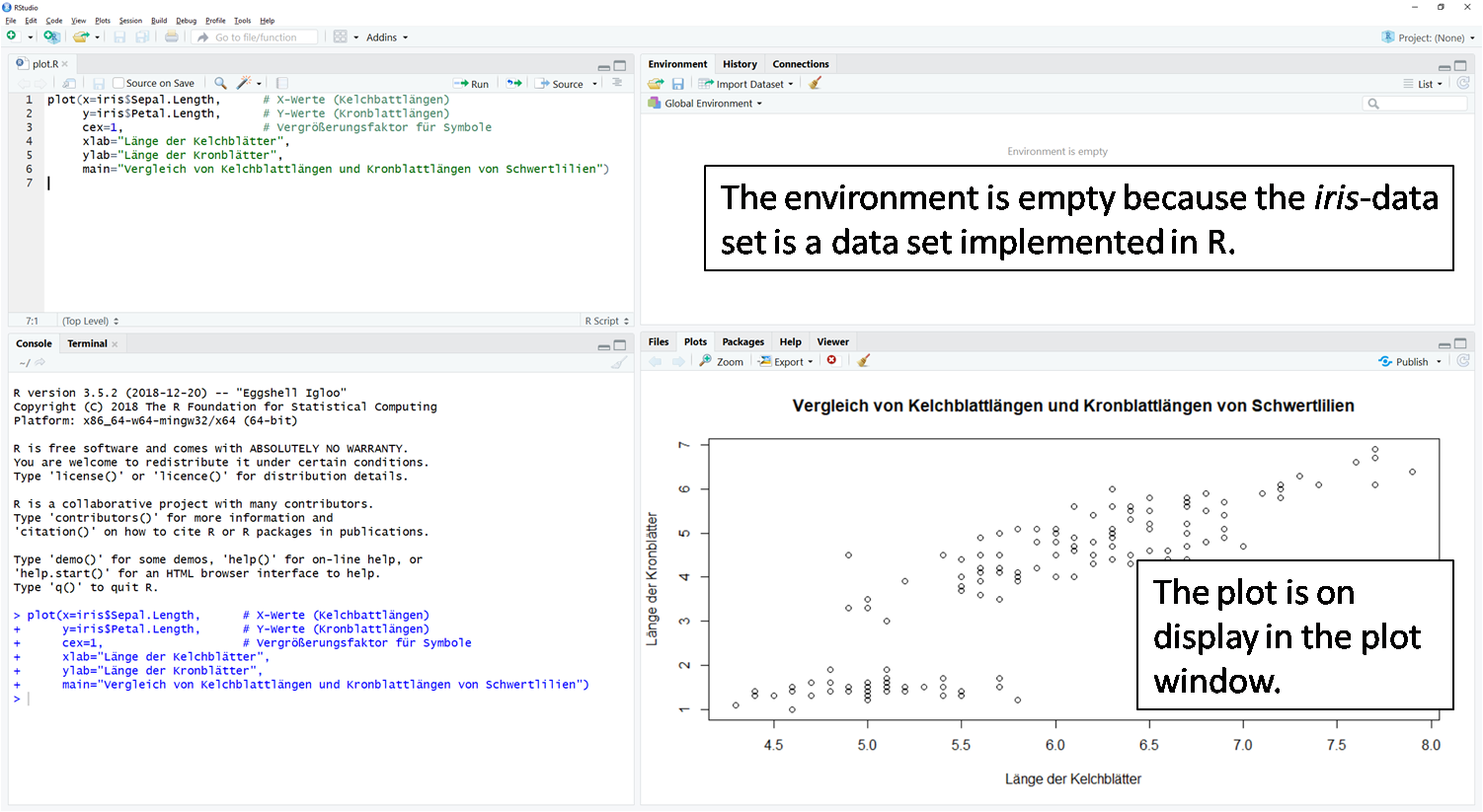
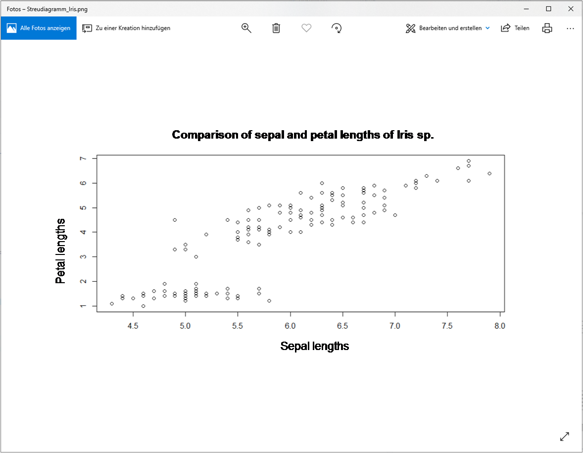
Here the in R implemented data set "iris" is plotted as a scatterplot. On the X-axis the calyx / sepal lengths and on the Y-axis the crown leaf / petal lengths are plotted.
-
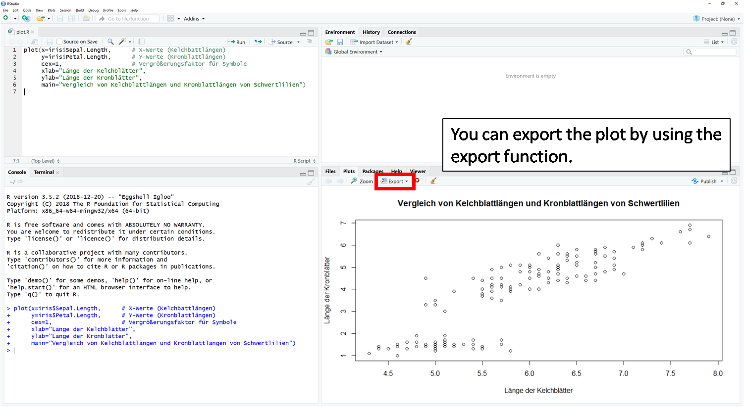
Via the tab "Export" you get to the export options of the created plot.
-
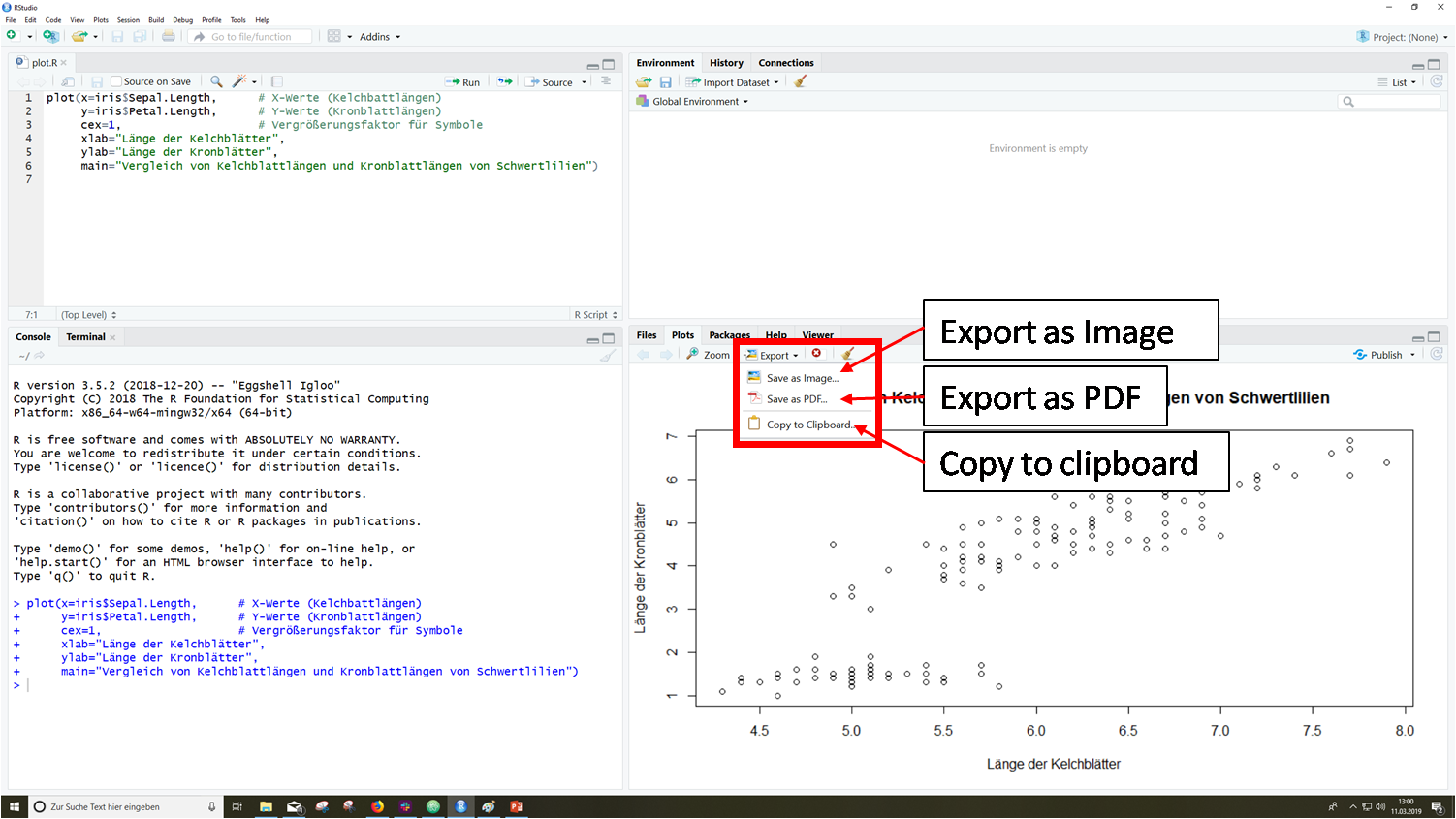
The three different export options are displayed here: 1. export in a graphic file format, 2. as a .pdf file or 3. the plot displayed is copied to the clipboard and you can paste it e.g., in a Word document with CTRL + V again.
-
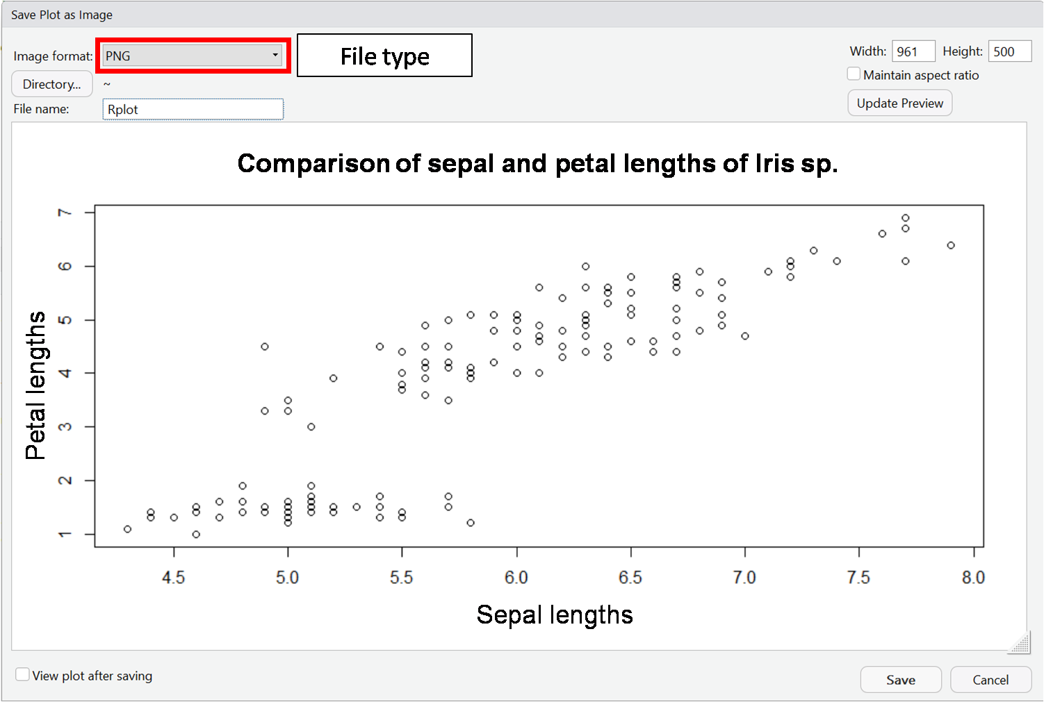
The plot is to be exported in a graphic file format. In the dialog window you can set the desired file format. Here the graphic should be exported as .png.
-
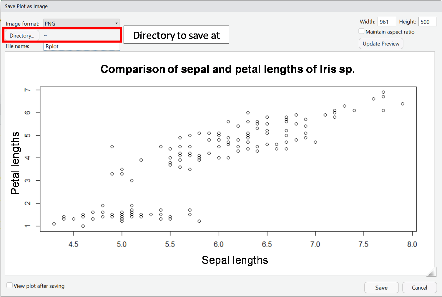
Here you select your desired storage location.
-
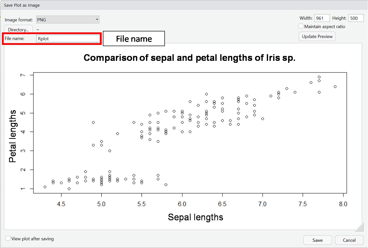
Here you enter the filename.
-
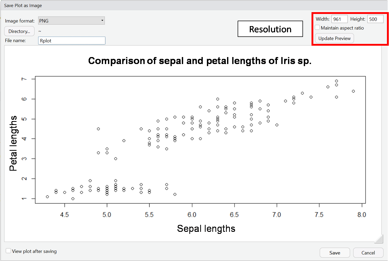
Here you can adjust the image size. In this example the default settings have been used.
-
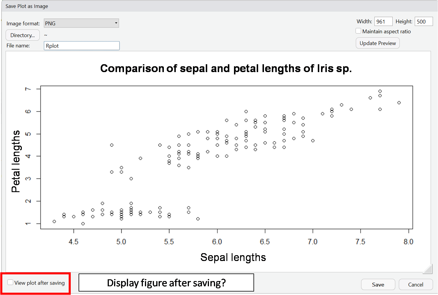
Here you can choose whether the graphic should be displayed after the export.
-
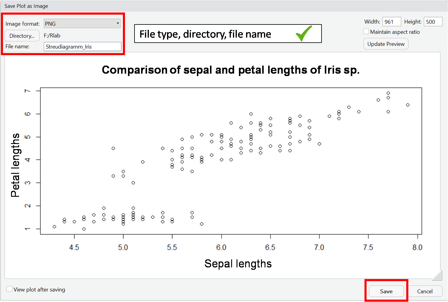
When the file format has been selected, the location determined and the file name assigned, you can click "Save".
-
The exported plot is displayed here.
Saving with the function png()
Furthermore you have the possibility to script the export.
- The first step is to create an empty file (here .png).
- In the second step follows the actual
plot()function. Here the plot is not displayed in the plot window. R keeps the plot in the invisible cache. - In the third step, the contents of the invisible cache are moved to the empty file from step 1 using the
dev.off()function.
Caution: If the function is repeated or another plot() function is executed, the file is overwritten each time. The last plot() command content before the dev.off() command is always moved into the file.
You want to try the export right now in R?
In the box you will find the code (which you can copy to R) under the Code tab and under the Console tab you will find the console output.
 # Empty png file is created.
 png("G:/Rlab/scatterplot_iris.png")
 }plot(x=iris$Sepal.Length,       # X-values (sepal lengths)
 y=iris$Petal.Length,            # Y-values (sepal lengths)
 cex=1,                          # Magnification factor for symbols
 xlab="sepal length",  # X-axis label
 ylab="petal length",   # Y-axis label
 main="Comparison of sepal lengths and petal lengths of Iris sp.")  # title of figure
 dev.off()
 # Empty png file is created.
 >png("G:/Rlab/scatterplot_iris.png")
 >
 >   plot(x=iris$Sepal.Length,      # X-values (sepal lengths)
 +        y=iris$Petal.Length,      # Y-values (sepal lengths)
 +        cex=1,                    # Magnification factor for symbols
 +        xlab="sepal length",
 +          ylab="petal length",
 +          main="Comparison of sepal lengths and petal lengths of Iris sp.")
 >
 >   dev.off()
 null device
 1
 >
You can see a step-by-step guide in the following slideshow:
-
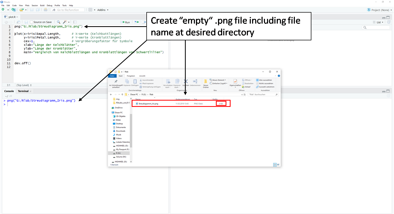
The first step is to create an "empty" png file. The name of the file is already assigned here.
-
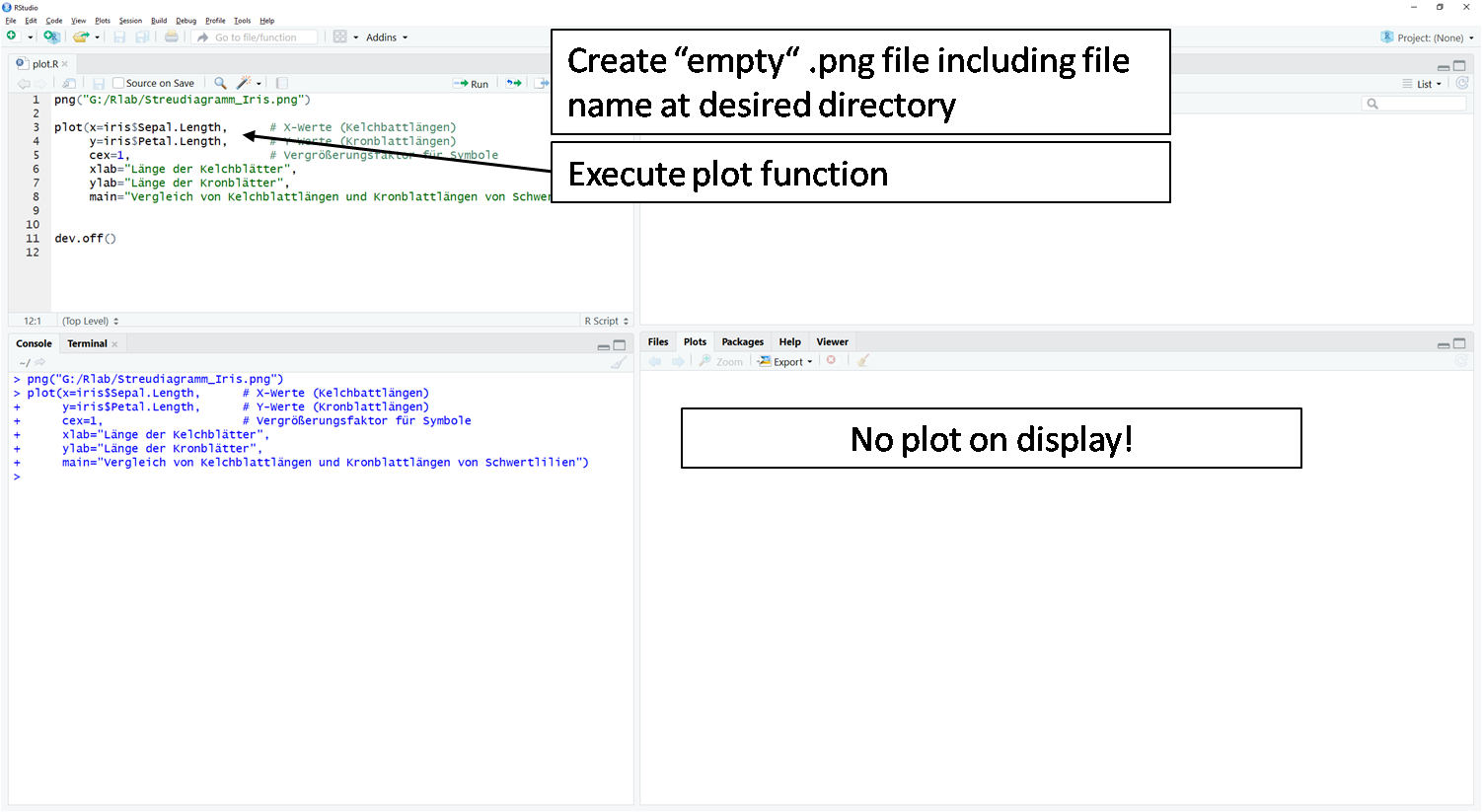
In the second step, the
plot()function is executed. But no plot appears in the plot window. The plot is placed internally on the clipboard. -
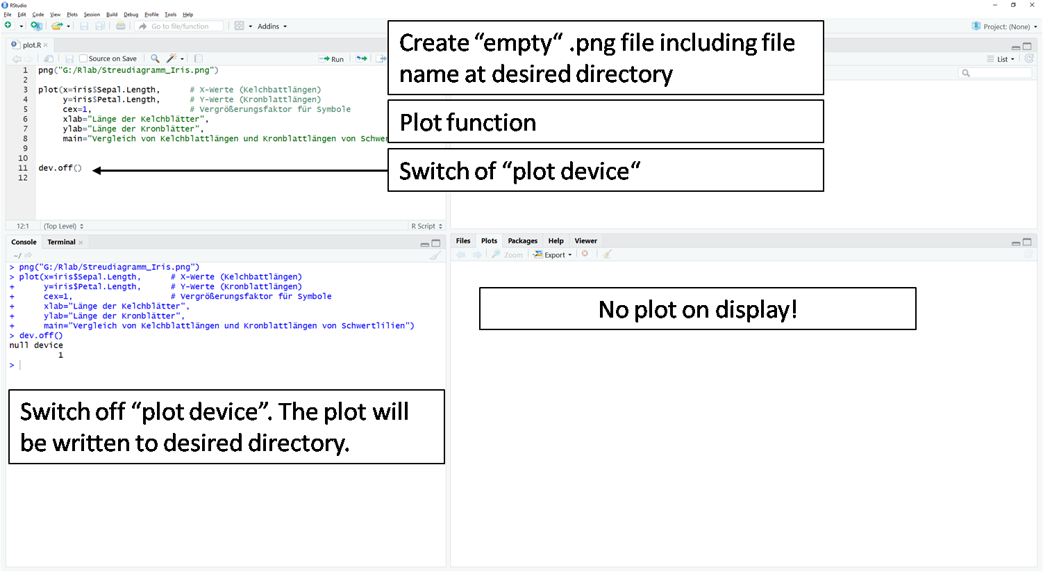
In the third step, the command
dev.off()is used to "flush" the plot from the clipboard into the empty .png file. The output in the "null device 1" console indicates that an internal graphics window has been closed. -
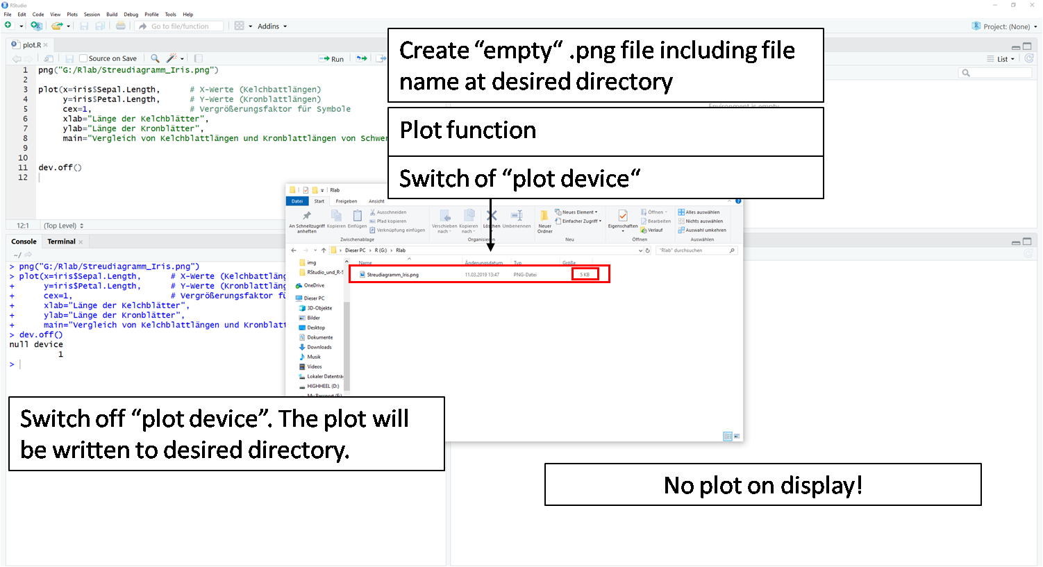
A look into the memory directory shows that the file now has a size of 5KB.
-

The plot was successfully exported from R and is displayed here in the Windows Photo Viewer.
Tips and tricks for saving tables
To export a table with results from R, use the write.table() function.
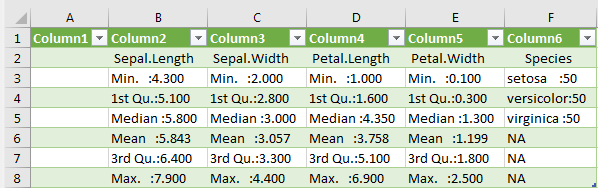
A very popular function for calculating descriptive statistics is the summary() function.
It outputs the parameters mean, median, minimum and maximum value, as well as the 1st and 3rd quartiles in a single step.
 descript_stats <- summary(iris)
> descript_stats
Sepal.Length    Sepal.Width     Petal.Length    Petal.Width          Species
 Min.   :4.300   Min.   :2.000   Min.   :1.000   Min.   :0.100   setosa    :50
 1st Qu.:5.100   1st Qu.:2.800   1st Qu.:1.600   1st Qu.:0.300   versicolor:50
 Median :5.800   Median :3.000   Median :4.350   Median :1.300   virginica :50
 Mean   :5.843   Mean   :3.057   Mean   :3.758   Mean   :1.199
 3rd Qu.:6.400   3rd Qu.:3.300   3rd Qu.:5.100   3rd Qu.:1.800
 Max.   :7.900   Max.   :4.400   Max.   :6.900   Max.   :2.500
Although a dataframe has been assigned here, it cannot be exported easily. Exporting is of course possible, but not in a respectable format:
write.table(deskript_stats, "G:/Rlab/descriptive_stat_iris.csv", dec=".", sep=";") If the file is opened in Excel, each cell also contains the statistical parameters. Here the table would have to be corrected manually.
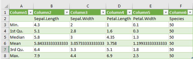
How's it easier?
With the combination of cbind and lapply the row labels are combined in one column and the descriptive statistics parameters are calculated for each column individually. So the dataframe can be exported as usual and the .csv file can be used for further applications.
 deskript_stats_1 <- do.call(cbind, lapply(iris, summary))
> deskript_stats_1
Sepal.Length Sepal.Width Petal.Length Petal.Width Species
Min.        4.300000    2.000000        1.000    0.100000      50
1st Qu.     5.100000    2.800000        1.600    0.300000      50
Median      5.800000    3.000000        4.350    1.300000      50
Mean        5.843333    3.057333        3.758    1.199333      50
3rd Qu.     6.400000    3.300000        5.100    1.800000      50
Max.        7.900000    4.400000        6.900    2.500000      50

write.table(deskript_stats_1, "G:/Rlab/summary_iris.csv", dec=".", sep=";")
If the .csv file is now opened in Excel, descriptive statistics parameters are located in a column below each other and the values in the cells.
Further useful hints can also be found in the "Exporting data to R" digital script at How do I export data in Comma-Separated-Values format? (in german only).
Further useful hints can also be found in the digital script for "Importing data in R" at Importing comma-separated values and text files in R (in german only).
Useful functions to check if your data has been imported correctly in R can also be found in the "Import data in R" digital script at Did my data import correctly in R? (in german only).
The art of scripting
Notations in R
When creating a script (name.R), special care should be taken when assigning object names.
There are some "unwritten laws" you should be aware of. An R script should be logical, well documented, and structured.
Not only can you remember your analysis steps after some time, but also others can understand your scripts and help you if necessary.
File name of script .R
No mutations (german umlauts ä, ö, ü) are allowed in script file names (name.R).
Also no special characters as !, +, - , #, *, … should be used.
GOOD: fit-models.R  (concise, meaningful, „telling” name)
BAD: stuff.R
Variable names
Variable names should be written in lower case and words should be divided by a dot or an underscore.
GOOD: avg_clicks (concise, meaningful, „telling” name)
OK: avgClicks
BAD: ac
Blanks
Binary operators =, +, -, <, >, ... should be enclosed by spaces.
No space should be placed before a comma, but always after it.
However: Spaces do not influence the processing of the code by R!
Quotes
Three types of quotes are part of the syntax of R: single (') and double (") quotation marks and the backtick (or back quote, `). In addition, backslash (\) is used to escape the following character inside character constants.
Character constants
Single and double quotes delimit character constants. They can be used interchangeably but double quotes are preferred (and character constants are printed using double quotes), so single quotes are normally only used to delimit character constants containing double quotes.
Backslash is used to start an escape sequence inside character constants. Escaping a character not in the following table is an error.
Single quotes need to be escaped by backslash in single-quoted strings, and double quotes in double-quoted strings.
(from R Documentation on Quotes)
For further explanations refer to e.g., DataCamp: Did my data import correctly in R? and R-help mailing list: Why double quote is preferred?.
library() vs require()
Both functions, library() and require() load R packages i.e., they "switch" installed packages on. In general, there is not much of a difference in everyday work.
However, require() is used inside functions, as it outputs a warning and continues if the package is not found, whereas library() will throw an error. When using require(), your code might yield different, erroneous results, without signaling an error.
Conclusion: require() is the wrong way to load an R package. Use library() instead.
Further, more detailed explanations and discussion:
- R-devel mailing list: require vs library
- Stack Overflow: What is the difference between require() and library()?
- Yihui Xie's blog: library() vs require() in R
Further, more extensive suggestions on the art of scripting:
- Wickham, H. (2017) Style guide [recommended, accessed March 09, 2019]
- Klein, M. C. (2018) INWT’s guidelines for R code [accessed March 09, 2019]
- Google Open Source (2018) Google’s R Style Guide [accessed March 09, 2019]
Your perfect R script
Beginning of an R script
It is recommended to always insert a header at the beginning of a R-script.
This header could look like this:
 ###################################################################
 # "INSERT TITLE OF SCRIPT"
 # "INSERT DATE"
 # "INSERT AUTHOR OR ORIGINAL URL"
 ###################################################################
 rm(list=ls()) # delete everything in the environment
 # important, since old files could interfere with the following calculations

 # # -----------------------------------------------------------------------


 # set Working directory
 setwd("INSERT_FILE_PATH")

 # loading packages
 library(ggplot2)


 # My first script ------------------------------------------------------


 # read / import data
 soil <- read.table("INSERT_FILE_PATH", header=T, sep=";", dec=".")


 # My first calculations -----------------------------------------------
 ....
 ...
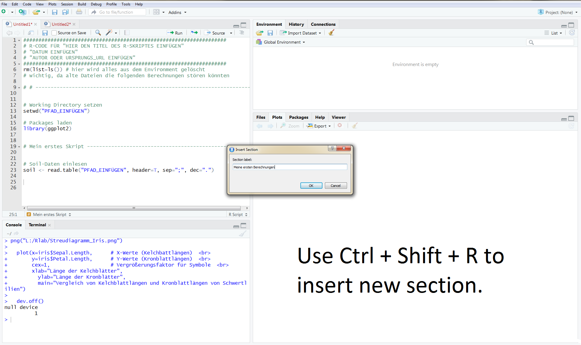
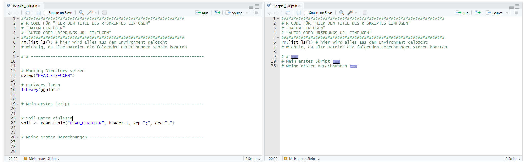
In the following picture you can see how the whole thing looks like in R. The use of at least ##### or ---- or ==== marks a new section within the script.
A small arrow will appear on the side of the script (in the script tab of RStudio) to collapse the code contained in this section. This allows you to hide code that has already been edited or is no longer needed, making the script easier to read.
The following keyboard shortcuts allow you to add and manage sections to your script.
Insert new section - Ctrl+Shift+R
Jump to next section - Shift+Alt+J
Collapse current section - Alt+L
Expand current section- Shift+Alt+L
Collapse all sections - Alt+O
Unfold all sections- Shift+Alt+O
With CTRL + SHIFT + R a new window appears, in which you can assign the section name.
Here you can see a comparison of the "unfolded" and "folded" sections.
Further, more extensive suggestions:
- Wickham, H. (2017) Style guide [recommended, accessed March 09, 2019]
- Klein, M. C. (2018) INWT’s guidelines for R code [accessed March 09, 2019]
- Google Open Source (2018) Google’s R Style Guide [accessed March 09, 2019]
Commenting your code
Compared to other statistical software such as Excel, SPSS or SAS, R has a decisive advantage: the comment function. With the # symbol you can write a comment for each step and thus document your learning process. Your attempts are by no means free or wasted time, but simply a learning process.
You will only learn R by trying out, combining and being able to "think like the program" on your own. Before you know it, dealing with R will become a matter of course.
The documentation of the individual steps in a script are your live saver! It is recommended to document as exactly as possible your individual steps and also the results.
Further useful hints can also be found in the "RStudio and R-Scripts" digital script at Advantages when working with R scripts (in german only) and in the "Importing data in R" digital script at Preparation of data (in german only).
Further, more extensive suggestions:
- Wickham, H. (2017) Style guide [recommended, accessed March 09, 2019]
- Klein, M. C. (2018) INWT’s guidelines for R code [accessed March 09, 2019]
- Google Open Source (2018) Google’s R Style Guide [accessed March 09, 2019]
Questions or remarks?
The RLab team is always grateful for suggestions and comments to improve this digital script! You can also ask questions about the content! Use the comments for all this!
The R Cheat Sheets
Since it is impossible to remember all the functions, you only need to know where to get the appropriate information! The R Cheat Sheet R Base offers a good overview of the essential functions and arguments of the package "base" which is implemented in every basic R installation.
This cheat sheet in particular is very helpful with the basic functionalities and working methods of vectors and other data formats, loops, mathematical functions and tests.
The cheat sheets on plotting graphs in R are also recommended. A good overview of the basic functions can be found in the R Base Graphics Cheat Sheet, everything about the formatting of the graphical representation can be found in the R Base Cheat Sheet Graph Sizes. On the website of RStudio you can find many more free R Cheat Sheets, separated by packages.
Summary
In this digital script you learned tips and tricks to ease your use of R.
Further tips can be found in other, more specific digital scripts (mostly in german).
Want to read a book to learn even more?
Check out the free version of Data science with R, authored by H. Wickham and G. Grolemund and recommended by user Ann Ca.
Questions or remarks?
The RLab team is always grateful for suggestions and comments to improve this digital script! You can also ask questions about the content! Use the comments for all this!